Zero Padding Calculator
Calculate how FFT zero padding changes display-bin spacing, peak readout precision, window bandwidth, timing, and update rate without confusing interpolation with true frequency resolution.
Load a common audio-analysis setup, then adjust the inputs. The calculator keeps the original window length separate from the padded FFT length so you can see what actually improves.
Calculation Breakdown
16,384
Padded FFT Points
85.3 ms
Original Window Time
23.4 fps
Analyzer Updates
4x
Display Interpolation
| Padding Factor | Padded Points From 4096 | 48 kHz Display Bin | What It Improves | What It Does Not Improve |
|---|---|---|---|---|
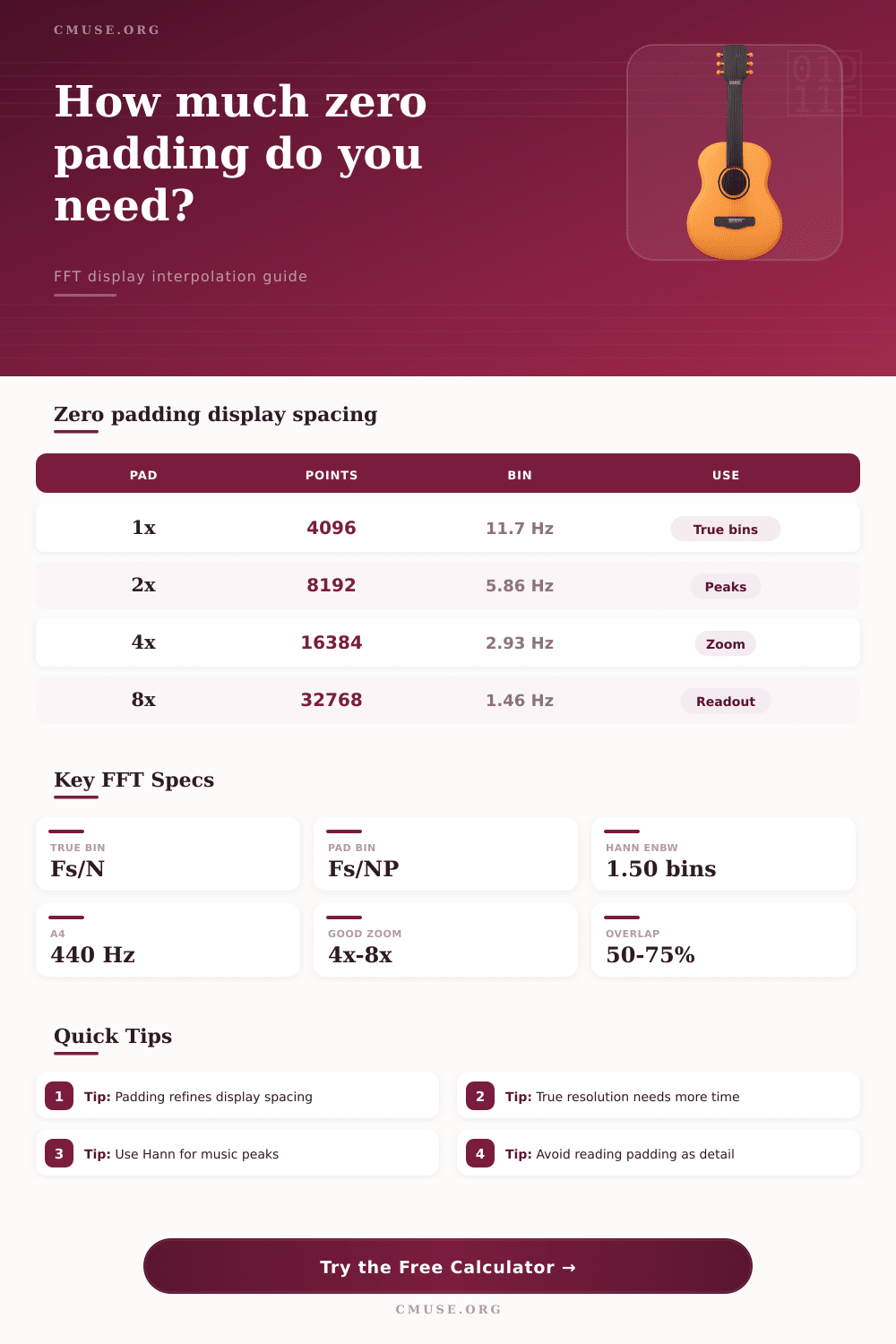
| 1x | 4,096 points | 11.719 Hz | Native FFT-bin readout | Peak shape sampling |
| 2x | 8,192 points | 5.859 Hz | Coarser peak interpolation | Resolving two close tones |
| 4x | 16,384 points | 2.930 Hz | Useful visual zoom for music peaks | Window main-lobe width |
| 8x | 32,768 points | 1.465 Hz | Smooth display curves and labels | Leakage or noise rejection |
| 16x | 65,536 points | 0.732 Hz | Dense graphing for reports | Extra physical information |
| Window | ENBW | Main Lobe | Highest Sidelobe | Best Zero-Padding Use |
|---|---|---|---|---|
| Rectangular | 1.00 bins | 2 bins | -13 dB | Coherent test tones only |
| Hann | 1.50 bins | 4 bins | -31 dB | Balanced musical peak display |
| Hamming | 1.36 bins | 4 bins | -43 dB | Single tones with less leakage |
| Blackman | 1.73 bins | 6 bins | -58 dB | Cleaner harmonic inspection |
| Blackman-Harris | 2.00 bins | 8 bins | -92 dB | Low sidelobe spectrum displays |
| Flat top | 3.77 bins | 10 bins | -93 dB | Amplitude readout, not close pitch |
| Scenario | Window | Typical Padding | Frequency Focus | Practical Readout Goal |
|---|---|---|---|---|
| Bass peak readout | 16,384 samples | 4x to 8x | 40 Hz to 120 Hz | Smoother peak maximum |
| Vocal formant view | 4,096 samples | 4x | 700 Hz to 3 kHz | Readable spectral curves |
| Guitar tuning zoom | 8,192 samples | 8x | 82 Hz to 330 Hz | Cent-level visual estimate |
| Live analyzer | 2,048 samples | 2x to 4x | Full range | Fast display response |
| Room mode sweep | 32,768 samples | 4x | 20 Hz to 200 Hz | Mode peak labeling |
| Hi-res spectrogram | 8,192 samples | 2x | Music detail | Balanced density and time |
| Method | Uses Zero Padding? | Strength | Weakness | Suggested Use |
|---|---|---|---|---|
| Nearest padded bin | Yes | Simple frequency labels | Still quantized to grid | Visual spectrum cursor |
| Parabolic peak | Helpful | Good with clear isolated peaks | Less stable on noisy peaks | Music tone readouts |
| Log-parabolic peak | Helpful | Often better for dB spectra | Depends on window shape | Analyzer peak labels |
| Phase-vocoder tracking | Optional | Strong frame-to-frame accuracy | Needs phase continuity | Pitch tracking and analysis |
What is this? A frequency analyzer shows you a peak rising then falling like a mountain range. Where’s the exact location of the bass note on the spectrum? Well, you pad zero to all your data, and now graph becomes smooth curves. It looks better. But has it added any information? No. That’s the source of most confusion with analyzing digital audio.
We think display resolution equals frequency resolution, which it doesn’t. This calculator distinguish between those two. This is important because this gives you two sets of information that your eyes and your ears can use differently. Eyes want lots of data points on the screen for smooth lines. Your ears wants enough data points in the time window to separate closely spaced notes. That’s why it takes a longer window (time) to hear any difference.
Zero Padding Makes Graphs Look Smoother But Does Not Add Real Information
If you put in the window length and sample rate, the calculator do the math for you and you don’t have to wonder whether what you’re seeing is actualy there or just interpolated points. True resolution come from the original recording length. No matter how much you pad it and no matter how many more zeros you throw at it, you cannot create information that was not captured in those initial samples.
In other words, if you recorded for 100 milliseconds, then you won’t be able to distinguish between two sounds separated by less than roughly 10 Hertz. Resolution is determined only by the original recording length. The hard limit comes from the equation: Fs/N. Padding out the recording doesn’t help. You simply end up stretching the data. But you’re never going to make up what wasn’t in the original samples. It’s like taking a really bad photo and zooming in on it, the pixels just get bigger but image doesn’t improve.
Without padding, you’ll have your native bin spacing, but window length determines how blurry the actual resolution is. With 4x padding, it will have display points at intervals of 2.75 Hertz if your native FFT bins are 11 Hertz apart. That can help you read your peak value more precisely. Without the padding, if a tone happens to fall midway between two native bins, then displayed amplitude will be less (due to scalloping loss). By filling in gaps with the padding to zero, you get closer to the peak by sampling spectral envelope more finely. You’ll see the tradeoff below in the breakdown section.
One more thing is the window function. For music purposes, you may prefer a Hann window, with a nice compromise between sidelobe leakage and main-lobe width. Its equivalent noise bandwidth is 1.5 bins wide though. Perhaps you prefer to look at weak harmonics alongside louder fundamentals? Try switching to the Blackman-Harris window; this greatly reduces sidelobes. The cost is a wider main lobe, meaning closely-spaced frequencies smear more then they would on another window. Padding reveals the shape of that wide lobe, but it doesn’t make it narrower.
Excessive padding is common among engineers trying to achieve more precise measurements than are possible. You pad 16x to resolve down to sub-Hertz steps when checking a guitar’s tuning. Sure! That makes graph look good. However, its underlying uncertainty is still dominated by noise floor and original window length. Even if you draw as many points as you want in between bins, if your peak is only 12 dB above the background noise level, you won’t know what your frequency was with any certainty. The calculator will estimate the error in your readout based off how much it stands out, so remember: A smooth curve on a noisy signal is an educated guess.
Other limitations include update rate and timing. Slower analyzers has longer windows. A 32,768 sample window produces noticeable delay if monitoring fast transients or live signals. In this case you may reduce the window to provide quicker response and back off with padding to recover some visual definition. The calculator indicates that this will restore the smoothness of display while degrading the low-frequency mode separation. This is a tradeoff between time and frequency.
Zero padding is useful for smoothing out the readout. It reduces the quantization effect on frequency resolution and smooths out the peaks with padding. But don’t think it’s going to sort out closely packed frequencies. Use the window length to hear what is there and use zero padding to see how it looks more clearly. The raw data contains the real truth while the smooth curves are just good for looking at, they should of been used to help understanding.