MLS Sequence Length Calculator
Calculate maximum length sequence order, samples, period time, impulse-response window, repeat averaging time, and acoustic path limits for MLS measurement work.
Pick a measurement scenario to load a practical MLS order and capture plan. The calculator checks whether the circular MLS period is long enough for the expected decay and room path.
For classic binary MLS, the order m is the shift-register length and the period contains every non-zero register state exactly once.
Calculation Breakdown
| MLS order | Sequence length | Period at 48 kHz | Frequency spacing | Typical measurement use |
|---|---|---|---|---|
| m = 10 | 1,023 samples | 21.3 ms | 46.92 Hz | Very short device checks and latency spotting. |
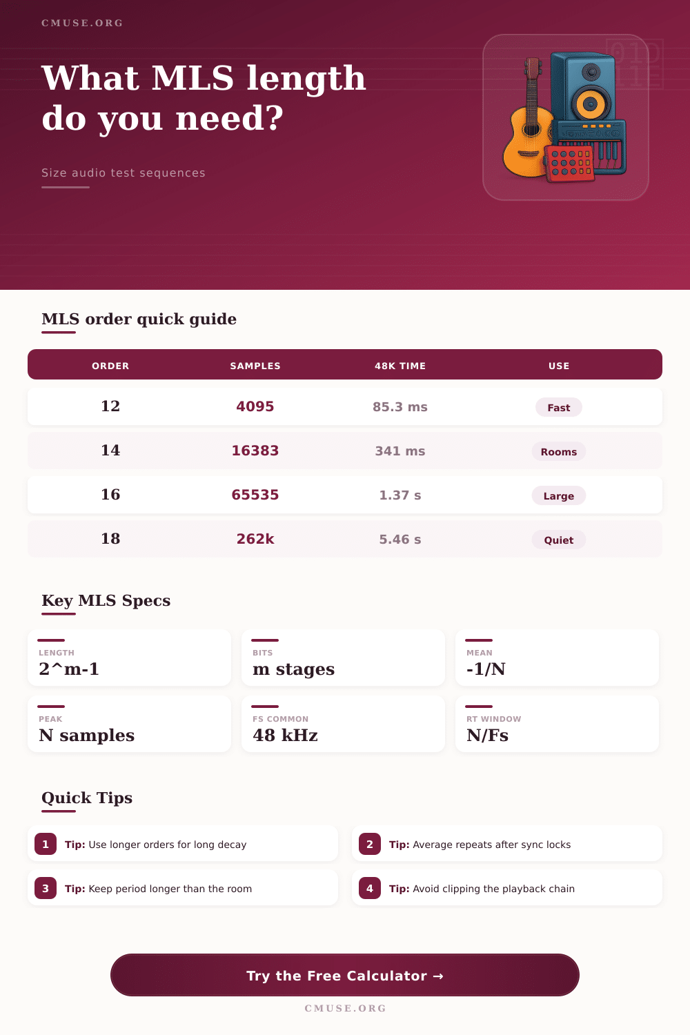
| m = 12 | 4,095 samples | 85.3 ms | 11.72 Hz | Fast loudspeaker close-mic checks. |
| m = 14 | 16,383 samples | 341 ms | 2.93 Hz | Small-room impulse windows and monitor tuning. |
| m = 16 | 65,535 samples | 1.37 s | 0.73 Hz | Room decay, studio RT work, and longer reflections. |
| m = 18 | 262,143 samples | 5.46 s | 0.18 Hz | Quiet measurements and reverberant spaces. |
| m = 20 | 1,048,575 samples | 21.85 s | 0.046 Hz | Long captures where repeat time is acceptable. |
| Method | Signal shape | Best strength | Watch item | Length planning note |
|---|---|---|---|---|
| MLS | Binary pseudo-random | Fast repeat averaging | Nonlinear distortion folds into the IR | Period must exceed the room response. |
| Log sweep | Sine sweep | Separates harmonic distortion | Needs deconvolution sweep file | Sweep duration sets SNR and low-frequency time. |
| Linear sweep | Sine sweep | Simple generator setup | Less efficient at low frequencies | Use longer sweeps for bass resolution. |
| Pink noise | Random noise | Realtime spectral balance | Not a direct impulse response | Average time controls display stability. |
| Measurement project | Suggested order | 48 kHz period | Path window | Starting repeats |
|---|---|---|---|---|
| Nearfield woofer response | m = 12 | 85 ms | 96 ft | 4 averages |
| Vocal booth reflection map | m = 13 | 171 ms | 192 ft | 8 averages |
| Small control room IR | m = 14 | 341 ms | 384 ft | 8 averages |
| Studio decay estimate | m = 16 | 1.37 s | 1,535 ft | 12 averages |
| Lecture hall response | m = 17 | 2.73 s | 3,071 ft | 16 averages |
| Reverberant sanctuary | m = 18 | 5.46 s | 6,142 ft | 16 averages |
| Order | One common feedback polynomial | Length | Autocorrelation peak | Use note |
|---|---|---|---|---|
| 10 | x^10 + x^3 + 1 | 1,023 | 1,023 | Good for electronics and nearfield checks. |
| 12 | x^12 + x^6 + x^4 + x + 1 | 4,095 | 4,095 | Short loudspeaker tests with quick repeats. |
| 14 | x^14 + x^5 + x^3 + x + 1 | 16,383 | 16,383 | Useful default for small-room MLS work. |
| 16 | x^16 + x^5 + x^3 + x^2 + 1 | 65,535 | 65,535 | Longer decay windows without very slow tests. |
| 18 | x^18 + x^7 + 1 | 262,143 | 262,143 | Large rooms or low ambient SNR. |
It would be simple if you could just generate some sound and see how long it takes until you hear an echo of yourself. That’s actualy quite complicated. You want a consistant signal. This lets you tell your room’s acoustic properties apart from other potential problems, such as the speakers themselves or electronics in your playback chain (i.e., system background hum).
One solution is called a Maximum Length Sequence (MLS), which are basically binary patterns (think digital white noise) that has ideal autocorrelation properties. That is, when you correlate what comes out back against itself you get a perfect impulse response. But there’s a catch: you have to use the right length.
How to Choose the Right MLS Length
What is the key variable? It’s the order of the sequence. At whatever sample rate you select, this means that calculator will tell you how many samples it can fit in a given period. This helps prevent common mistakes. Higher order result in a longer period. There is more elapsed time between the start of one signal repeat and the next before it starts to wrap around on itself.
Late energy folds back into beginning of the impulse response if the MLS period is too short for your room’s long decay tail. Then you end up measuring ghosts. The sequence length isn’t aligned with what acoustically exists in space. Start by considering the decay time.
Twelve or fourteen are usually plenty for a small vocal booth with lots of absorption; it makes measurement fast while reducing exposure to system drift. Attempting the same order in a large reverberant hall cut off the tail end before it has a chance to die out. The trick here is getting more than enough time so that sound doesn’t matter anymore different than your noise floor.
If there are long reflection paths or a delayed speaker array, then you also need to be sure that overall path length fits into the sequence window. Averaging plays an overlooked role. Once the sync lock is stabilized, you can increase number of measurements (the signal-to-noise ratio improves). However, the initial few cycles may be contaminated by level adjustments or startup transients; the tool discards these warm-up periods. It makes a difference if you attempt to resolve fine details of frequency response, and throwing away the first few does clean up result.
And this all depends on sample rate too. For example, most audio work runs at forty-eight kilohertz, because that gives enough bandwidth to cover audible frequencies without requiring excess storage space. Higher rates give more resolution but increase time it takes to process any single command (which may not be worth the extra work). The calculator will show you total time required to capture and help match those factors.
Twenty seconds on your test? Chances are you’re working with some high averaging count or an exceedingly long sequence. MLS treats nonlinear distortion differently than sweeps do. Early artifacts is harmonic distortions that fold back into the impulse response through the amplifier or speaker. If your playback chain is clean, this isn’t necessarily bad and can be an indicator of what to listen for.
To help ensure a clean response, keep levels moderate so no clipping occurs on the peak of binary sequence. Most people tend to crank up the volume thinking it’s helping them; it doesn’t and usually just breaks the straight-line assumption. In reality, selecting the proper MLS length is a compromise between dynamic range, resolution and time.
It must be short enough to record the complete acoustic picture but not so short that it miss information. It must be long enough to average out unwanted ambient noise without wasting time. You should of checked your settings first. In a usual recording scenario, the reference table provides a starting point, such as when comparing nearfield checks to room decay analysis.
For generic studio work, start with something reasonable such as fourteen. That’s a decent compromise between window size and speed. Tweak upwards if it’s wrapping and downwards if all you’re after is a quick frequency check on a driver. Remember: this isn’t about getting every metric perfect; it’s about having a consistant representation of the space.
After capturing the clean impulse response, the rest falls out naturaly; measure the room, not the artifacts of your test setup.