FIR Filter Calculator
Estimate tap count, window behavior, linear-phase delay, coefficient memory, and DSP workload for audio FIR filters using practical window-method formulas.
🎛 FIR Design Presets
📐 Filter Inputs
Coefficient Preview
⚙ Current Design Snapshot
📊 FIR Window Reference
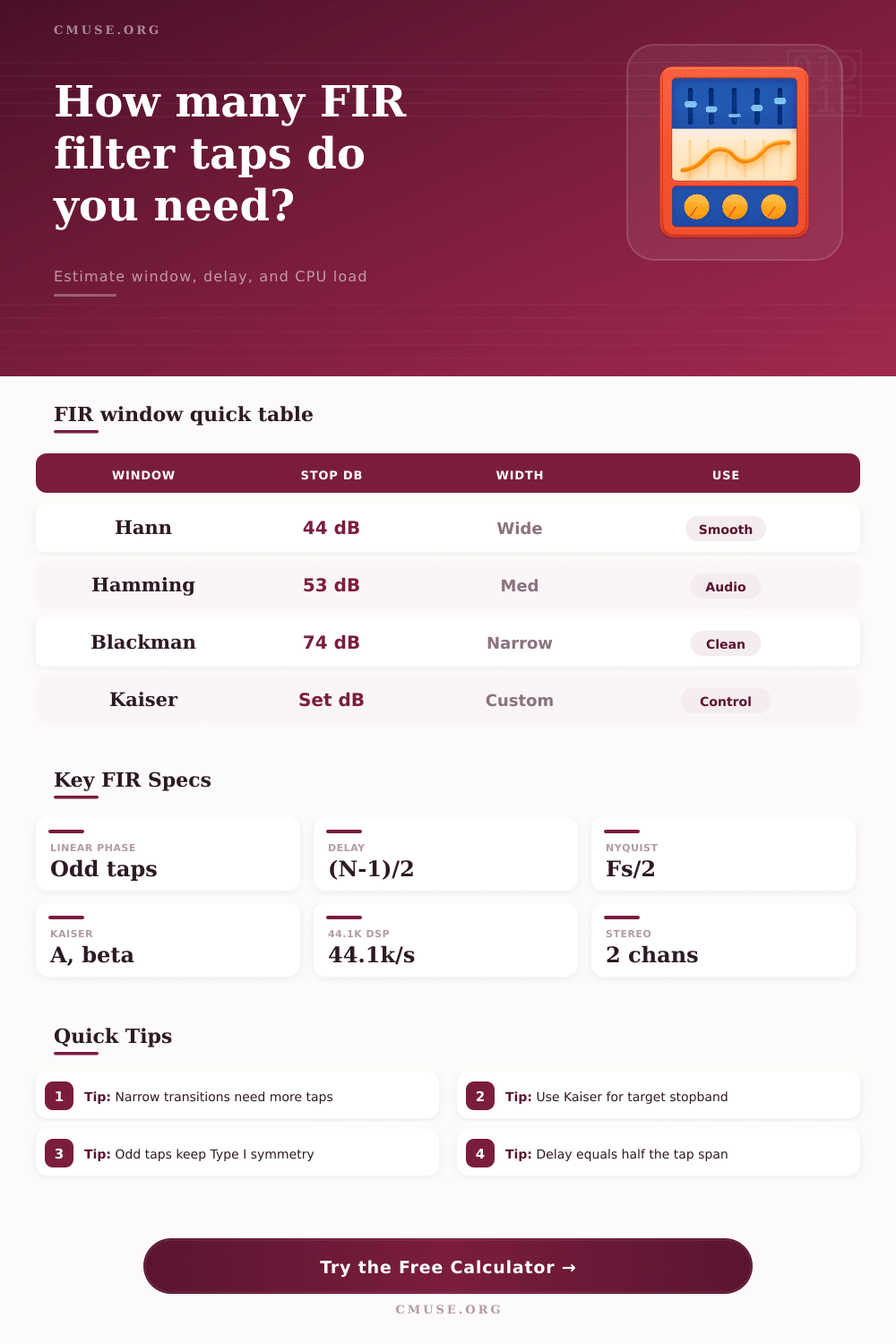
| Window | Typical Stopband | Transition Estimate | Best Use |
|---|---|---|---|
| Rectangular | About 21 dB | N ≈ 0.9 Fs / Δf | Fast estimates, narrowest transition, high ringing. |
| Hann | About 44 dB | N ≈ 3.1 Fs / Δf | Smooth audio shaping where rejection is moderate. |
| Hamming | About 53 dB | N ≈ 3.3 Fs / Δf | General audio FIR filters and compact EQ sections. |
| Blackman | About 74 dB | N ≈ 5.5 Fs / Δf | Cleaner rejection when extra delay is acceptable. |
| Blackman-Harris | About 92 dB | N ≈ 7.0 Fs / Δf | Low side-lobe spectral work and mastering filters. |
| Kaiser | User target | N from A and Δω | Designs that need adjustable attenuation and delay tradeoffs. |
🎚 Common FIR Audio Scenarios
| Scenario | Sample Rate | Transition | Typical Window | Design Note |
|---|---|---|---|---|
| Streaming low-pass | 44.1 to 48 kHz | 2 to 5 kHz | Hamming or Kaiser | Keeps tap count short while removing ultrasonic content. |
| Subwoofer crossover | 48 to 96 kHz | 20 to 80 Hz | Kaiser | Very narrow transitions create long delay quickly. |
| Hum notch | 44.1 to 96 kHz | 2 to 10 Hz | Kaiser | Sharp 50 or 60 Hz rejection may need thousands of taps. |
| Speech band-pass | 16 to 48 kHz | 100 to 400 Hz | Hann or Hamming | Moderate rejection is often enough for voice cleanup. |
| Mastering linear phase | 96 to 192 kHz | 4 to 12 kHz | Blackman-Harris | High stopband rejection can be worth added latency offline. |
📘 Formula Breakdown
| Quantity | Formula | Meaning | Audio Impact |
|---|---|---|---|
| Normalized transition | Δf / Fs | Transition bandwidth as cycles per sample. | Smaller values demand longer FIR filters. |
| Kaiser beta | 0.1102(A - 8.7) above 50 dB | Shape parameter for the Kaiser window. | Higher beta lowers side-lobes and widens transition. |
| Group delay | (N - 1) / (2 Fs) | Linear-phase latency before block buffering. | Important for live monitoring and instrument processing. |
| Direct MAC rate | N × Fs × channels | Multiplications per second for direct convolution. | Long filters can push small embedded DSP chips hard. |
| Memory | N × channels × bits/8 | Coefficient storage before sample history buffers. | Small, but grows with many channels or double precision. |
🧪 Practical Tap Ranges
| Tap Count | Latency at 48 kHz | Direct Stereo Load | Typical Placement |
|---|---|---|---|
| 31 taps | 0.31 ms | 3.0M mult/s | Tone shaping, gentle anti-aliasing, small devices. |
| 127 taps | 1.31 ms | 12.2M mult/s | Common real-time audio FIR, EQ, crossover tasks. |
| 511 taps | 5.31 ms | 49.1M mult/s | Linear-phase correction where delay is acceptable. |
| 2047 taps | 21.31 ms | 196.5M mult/s | Sharp notches, room correction, FFT partitioned convolution. |
Finite Impulse Response (FIR) filter are used to process audio signals. FIR filters must find a balance between the precision of the frequency response of the filter and the speed at which it can perform its calculation. FIR filters must decide between a sharp cutoff of the unwanted frequency in the signal and a low amount of latency in the processed signal.
A sharp cutoff allow for more effective separation of the noise from the audio signal, but requires a higher number of taps. The number of taps in an FIR filter determine the transition width of the signal. The transition width is the range of frequencies between the passband and the stopband of the filter.
FIR Filter Choices: Accuracy, Delay and Processing Power
A narrow transition width allow for high precision in the frequency response, but requires a higher number of taps. An increased number of taps increase the group delay of the signal. The group delay of a signal is the time it takes for that signal to pass through the FIR filter.
High group delay create latency in the audio signal. High latency can lead to problems in live sound performance. Therefore, the sound engineer must make a decision as to whether the precision of the FIR filter is worth the latency that high tap counts introduce into the signal.
Window functions can be used to modify the FIR filter to prevent mathematical error. If the mathematical function is simply truncated to create the FIR filter, it will introduce errors into the frequency response of the signal that are referred to as the Gibbs effect. The Gibbs effect create unwanted oscillations in the audio signal.
Using a window function such as a Hann window to smooth the FIR filter’s response can prevent these oscillations. The Hann window may, however, not provide enough rejection in the stopband of the filter. If deep stopband rejection is required, a Blackman window or an Kaiser window can be used.
The Kaiser window can be tuned to provide a specific level of attenuation in the stopband. Thus, the Kaiser window is useful for creating filters that must have a specific level of decibel rejection in there stopband. The transition width of a FIR filter is one of the variables that determine the computational cost of implementing the filter in hardware.
If the transition width is made very narrow, such as from 20 kHz to 19 kHz, the number of taps required to create the FIR filter will significantly increases. As a result, the computational cost of the FIR filter will significantly increase as well. Each tap to the FIR filter require the multiplication and addition of each sample of audio data.
The computational cost of performing such operations on each sample is the processing power of the digital signal processor (DSP). If a wide transition width is used instead, the number of taps required for implementation of the FIR filter will decrease. Fewer taps reduces the processing power required of the DSP to implement the FIR filter.
Computational resource and memory are two resources that can be required to implement an FIR filter. A DSP in a desktop computer can handle any number of taps. However, an embedded chip or DSP may struggle with high tap counts.
If the number of taps is too high for a DSP, that chip may “glitch” or become unstable while attempting to complete the million of operations that are required each second. Another resource to consider is the memory required to store the coefficients of the FIR filter. If many FIR filters are implemented on many audio channels, the coefficients will take up memory in the cache of the processor.
Accessing memory in the cache is fast, but using too much of the cache memory slow the processing loop. The coefficients of the FIR filter can be of any word length. If 16-bit numbers are used, the processing will be less precise than if 32-bit numbers were use.
The sound engineer requires a decision as to what is the most important aspect of the filter in the design of an FIR filter. For example, is a steeper slope in the frequency response of the filter more important than a lower group delay in the audio signal? Another decision that must be made is whether deep stopband rejection is more important than a low computational cost of implementing the FIR filter.
Each of these variable can be understood and their effects on the design of an FIR filter can be considered. Based on these understandings, it is possible to design an FIR filter that meets the requirements of a given sound engineer and sound mixing projects.