Audio Graphing Calculator
Plan waveform, FFT, spectrum, and decibel graph settings from sample rate, display size, frequency range, and amplitude floor.
🎚 Quick Presets
📈 Graph Inputs
FFT bin spacing uses sample rate divided by FFT size. The highest valid plotted frequency is limited by the Nyquist frequency, which is half the sample rate.
🎶 Spec Comparison Grid
📊 Sample Rate Reference
| Sample Rate | Common Use | Nyquist Frequency | One Millisecond Samples |
|---|---|---|---|
| 16 kHz | Speech capture and call analysis | 8 kHz | 16 samples |
| 44.1 kHz | CD audio and music distribution | 22.05 kHz | 44.1 samples |
| 48 kHz | Video, broadcast, podcasts, games | 24 kHz | 48 samples |
| 96 kHz | High-resolution mix and mastering checks | 48 kHz | 96 samples |
| 192 kHz | Measurement and ultrasonic inspection | 96 kHz | 192 samples |
🔬 FFT Size Reference
| FFT Size | 48 kHz Bin Width | 96 kHz Bin Width | Best Use |
|---|---|---|---|
| 512 | 93.75 Hz | 187.50 Hz | Fast transient view |
| 1024 | 46.88 Hz | 93.75 Hz | Drum and rhythm editing |
| 2048 | 23.44 Hz | 46.88 Hz | Speech and quick spectrum checks |
| 4096 | 11.72 Hz | 23.44 Hz | General mix analysis |
| 8192 | 5.86 Hz | 11.72 Hz | Low-frequency mix balancing |
| 16384 | 2.93 Hz | 5.86 Hz | Mastering and bass detail |
| 32768 | 1.46 Hz | 2.93 Hz | Noise floor and fine measurement |
📐 Window Function Comparison
| Window | Main Lobe | Leakage Control | Recommended Graph Use |
|---|---|---|---|
| Rectangular | Narrowest | Low | Exact looped tones and quick transients |
| Hann | Moderate | Good | General music spectrum graphs |
| Hamming | Moderate | Good | Speech, voice, and stable instruments |
| Blackman | Wider | Very high | Mastering, noise, and low-level detail |
🎛 Common Audio Graph Presets
| Graph Task | Window | FFT | Display Range |
|---|---|---|---|
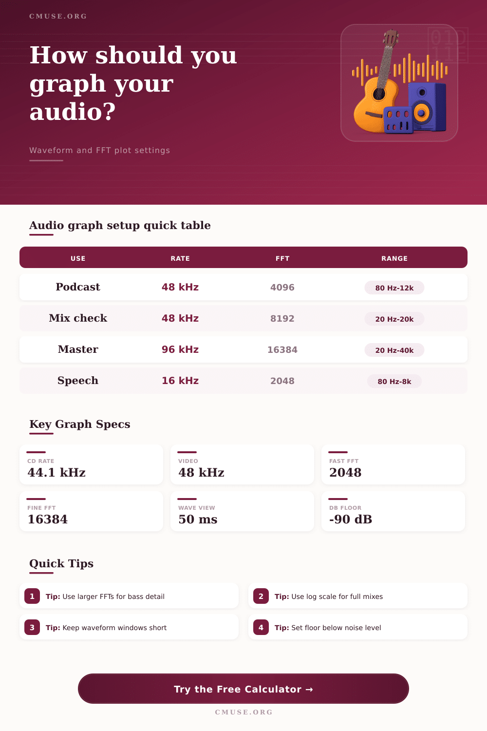
| Podcast voice cleanup | 25-60 ms | 2048 | 80 Hz to 12 kHz |
| Full mix spectrum | 50-100 ms | 4096 or 8192 | 20 Hz to 20 kHz |
| Kick transient zoom | 5-15 ms | 512 or 1024 | 40 Hz to 10 kHz |
| Bass note inspection | 150-500 ms | 8192 or 16384 | 20 Hz to 1 kHz |
| Noise floor check | 250-1000 ms | 16384 or 32768 | 20 Hz to 20 kHz |
🔎 Axis Scale Comparison
| Scale | Pixel Meaning | Strength | Use When |
|---|---|---|---|
| Linear | Equal Hz per pixel | Clear technical spacing | Measuring tones, harmonics, and test signals |
| Logarithmic | Equal ratios per pixel | Matches musical pitch spacing | Viewing mixes, instruments, and broad spectra |
| Waveform time | Equal time per pixel | Shows edits and transients | Checking clicks, timing, and envelopes |
| dB amplitude | Equal dB steps | Shows quiet detail | Comparing noise, tails, and dynamic range |
Spectral analyzers allows individuals to visualize the frequencies of an audio file. However, the settings on the analyzer will determine the accuracy of that visual data. Many individual will use the default settings on a spectral analyzer.
However, using the default settings can produce inaccurate data because the spectral analyzer must make a trade-off between time resolution and frequency resolution in order to derive the correct data. Therefore, understanding the relationship between time and frequency will allow individuals to use the spectral analyzer correct. The size of the Fast Fourier Transform (FFT) determines the frequency resolution of a spectral analyzer.
How to Use a Spectral Analyzer
Using a larger FFT will provide better frequency resolution because a larger FFT will capture more samples of audio over a longer time period. Furthermore, using a larger FFT allows the analyzer to differentiate between two close frequencies. If the FFT size is too small, the bin width will be too wide.
This make it likely that the spectral analyzer will produce a resonant frequency peak at the wrong frequency value; instead of the correct value for the frequency of interest. Spectral analyzers use window functions to process the audio samples. These window functions are necessary because the audio samples dont always begin and end neatly for the analyzer.
By cutting the audio signal abruptly, the spectral analyzer will show high frequencies that are not naturaly within the sound sample. This is called spectral leakage. To avoid spectral leakage, the spectral analyzer can use a window function like the Hann window or the Blackman window.
These window functions will fade the beginning and end of the audio samples. By using these window functions, the spectral analyzer can derive a cleaner graph of the sound sample. The needs of the individual using a spectral analyzer will change based off the type of sound being analyzed.
Using a long FFT window is helpful for analyzing sustained sounds to get high frequency resolution. However, it is not helpful for transient sounds because the transient sound will be averaged over a longer time period. For transient sounds, the FFT window will need to be short enough to catch the transient hit but long enough to include the fundamental frequency of the sound.
The axis scales on a spectral analyzer can be set to a linear scale or a logarithmic scale. A linear scale will produce the technically accurate data for the sound sample. The linear scale will be helpful for laboratory measurements of sound samples.
It will also be helpful for tuning a sine wave. However, human hearing isnt a linear scale. Humans hear in octaves.
Therefore, the logarithmic scale is more helpful than mixing music. The logarithmic scale will mimic the way humans hear sounds. Using this scale will make the graph expanded in the bass region but compressed in the high frequencies.
The amplitude floor will determine the detail visible on the spectral analyzer graph. If the amplitude floor is set too high, the bottom of the graph will be clipped, and there will be an inability to view the subtle details in the sound sample. If the amplitude floor is set too low, individuals will begin to see the digital noise that is present in the hardware.
This will be distracting from the sound being analyzed. Finding the correct amplitude floor will allow individuals to see the tail of a reverb return or the hiss of a preamp without seeing irrelevant data. Spectral analyzers will never allow individuals to have perfect time resolution and frequency resolution at the same time.
The analyzer will have to make a trade-off between the two. If time resolution is more important than frequency resolution, the analyzer will be able to derive when a sound occurred but will have less precision in the frequency value. However, if frequency resolution is more important than time resolution, the analyzer will have a precise value for the frequency of the sound but will have less precision with when that sound occurred.
By adjusting the settings for the FFT size, window function, axis scale, and amplitude floor, the spectral analyzer will be able to produce an accurate visual representation of the audio being analyzed.