Chirp Rate Calculator
Calculate linear Hz-per-second sweep rate, logarithmic octave and cent rate, marker frequency, total cycles, sample count, and Nyquist margin for audio chirps and measurement sweeps.
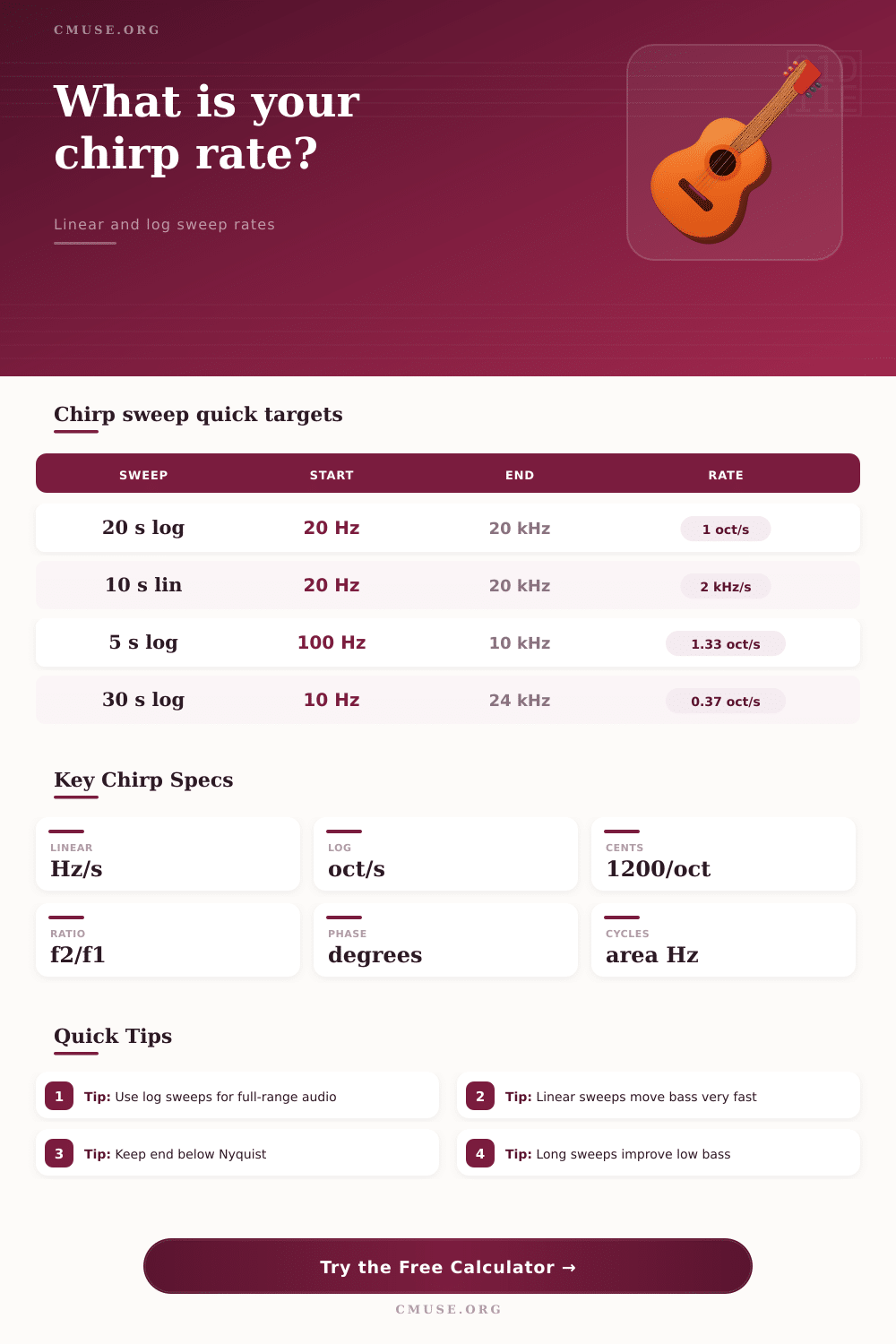
Choose a real sweep scenario, then refine the frequency span, duration, curve, sample rate, and marker time. Linear chirps move by a constant number of Hz each second; log chirps move by a constant musical ratio each second.
Linear formula: f(t) = f1 + (f2 - f1)t/T. Log formula: f(t) = f1 x (f2/f1)^(t/T). Total linear cycles equal T(f1 + f2)/2; total log cycles equal T(f2 - f1)/ln(f2/f1).
Calculation Breakdown
| Quantity | Linear chirp | Logarithmic chirp | Units | Why it matters |
|---|---|---|---|---|
| Instant frequency | f1 + kt | f1 x r^(t/T) | Hz | Determines the tone heard at any point in the sweep |
| Primary rate | k = (f2 - f1) / T | log2(f2/f1) / T | Hz/s or oct/s | Shows whether the sweep moves evenly by frequency or ratio |
| Total cycles | T(f1 + f2) / 2 | T(f2 - f1) / ln(f2/f1) | Cycles | Equivalent to the area under the frequency-time curve |
| Midpoint frequency | (f1 + f2) / 2 | sqrt(f1 x f2) | Hz | Explains why a log sweep spends more time in low octaves |
| Musical feel | Fast through bass | Even per octave | Ratio | Log sweeps track pitch spacing more naturally |
| Audio task | Typical span | Duration | Curve | Approximate rate | Practical note |
|---|---|---|---|---|---|
| Full-range room sweep | 20 Hz to 20 kHz | 10 to 30 s | Log | 0.33 to 1.0 oct/s | Longer sweeps give low frequencies more cycles |
| Subwoofer alignment | 10 Hz to 200 Hz | 20 to 60 s | Log | 0.07 to 0.22 oct/s | Slow movement helps reveal modal peaks and nulls |
| Fast device check | 20 Hz to 20 kHz | 2 to 5 s | Linear | 4 to 10 kHz/s | Good for quick functional checks, less ideal for bass detail |
| Tweeter band sweep | 2 kHz to 20 kHz | 5 to 10 s | Log | 0.33 to 0.66 oct/s | Confirms high-frequency response without wasting bass time |
| Instrument pickup test | 80 Hz to 8 kHz | 8 to 15 s | Log | 0.44 to 0.83 oct/s | Covers fundamentals and harmonics at a musical pace |
| Filter trace sweep | 100 Hz to 10 kHz | 5 to 20 s | Either | 0.33 to 1.33 oct/s | Use linear when the filter spec is in fixed-Hz bandwidth |
| Sweep | 25% time | 50% time | 75% time | Linear midpoint | Log midpoint |
|---|---|---|---|---|---|
| 20 Hz to 20 kHz | Linear 5.02 kHz, log 112 Hz | Linear 10.01 kHz, log 632 Hz | Linear 15.01 kHz, log 3.56 kHz | 10.01 kHz | 632 Hz |
| 10 Hz to 200 Hz | Linear 57.5 Hz, log 21.1 Hz | Linear 105 Hz, log 44.7 Hz | Linear 152.5 Hz, log 94.6 Hz | 105 Hz | 44.7 Hz |
| 100 Hz to 10 kHz | Linear 2.58 kHz, log 316 Hz | Linear 5.05 kHz, log 1 kHz | Linear 7.53 kHz, log 3.16 kHz | 5.05 kHz | 1 kHz |
| 2 kHz to 20 kHz | Linear 6.5 kHz, log 3.56 kHz | Linear 11 kHz, log 6.32 kHz | Linear 15.5 kHz, log 11.25 kHz | 11 kHz | 6.32 kHz |
| Sample rate | Nyquist limit | Safe sweep end | Samples in 10 s | Samples in 30 s | Common use |
|---|---|---|---|---|---|
| 44.1 kHz | 22.05 kHz | 20 kHz | 441,000 | 1,323,000 | Music playback and CD-rate checks |
| 48 kHz | 24 kHz | 22 kHz | 480,000 | 1,440,000 | Video audio, interfaces, and room measurement |
| 96 kHz | 48 kHz | 40 kHz | 960,000 | 2,880,000 | Extended-bandwidth hardware testing |
| 192 kHz | 96 kHz | 80 kHz | 1,920,000 | 5,760,000 | Ultrasonic measurement and lab sweeps |
| Type | Rate behavior | Best for | Watch point | Frequency-time shape | Use when |
|---|---|---|---|---|---|
| Linear up-sweep | Constant Hz/s | Filter bandwidths, fast hardware scans | Bass passes quickly | Straight line | Specifications are measured in fixed Hz |
| Linear down-sweep | Constant negative Hz/s | Checking hysteresis or direction-sensitive displays | Same bass-time issue | Straight falling line | You need high-to-low motion |
| Log up-sweep | Constant octaves/s | Loudspeaker, room, and musical-response sweeps | Needs positive start and end frequencies | Exponential curve | Each octave deserves similar attention |
| Log down-sweep | Constant negative octaves/s | Reverse response checks and special test tones | End time can feel crowded in bass | Exponential fall | You want ratio spacing from high to low |
| Segmented chirp | Rate changes by band | Custom lab sweeps | Requires splicing or generated sections | Piecewise | One band needs extra resolution |
A linear sweep move forward by a constant number of hertz per second. On paper, this seems perfectly reasonable. From zero to ten seconds, if you’re starting at twenty hertz and ending at twenty kilohertz, then there’s a clear sense of evenness.
But human perception of pitch is not linear. Instead, it’s logarithmic. This means our ears perceive the next step up as being equally large whether its an octave jump (from two hundred to four hundred hertz) or an octave jump twelve octaves higher (four thousand to eight thousand hertz). In terms of pure distance covered with each step, the latter jump covers three thousand and eight hundred hertz. Yet we hear it as equivalent to the former jump.
Why Use a Logarithmic Sweep for Audio Testing
What that means is that a linear sweep whizzes through the lower frequencies where speaker resonances and room modes resides. Then it barely brushes past the bass and races upward into the mids and highs. That’s where details are that make all the difference when it comes to sound quality.
Each octave gets the same proportion of the overall sweep time, achieved through use of a logarithmic curve. The tool will take your preferred frequency span and duration and calculate the parameters needed to get it done. It also figures out exactly how many octaves per second so you’re getting a constant resolution throughout the range people can hear. That’s essential if you’re measuring room modes or loudspeaker response. Those issues is often expressed as a function of where they fall within a certain musical interval, not at some arbitrary number of hertz. So if you want to make a ten-second sweep from twenty to two-hundred hertz, the result should show a balanced view of two hundred to four-thousand hertz in that same time span.
The page has a reference table to explain this neatley for typical situations. The other real-world trade-off has to do with length. Longer sweeps has better signal-to-noise because they spread out the energy across more cycles. This benefits deconvolution algorithms by producing sharper impulse response recoveries with less phase error, this also makes standing wave and phase errors detectable. But long files take up more disk space and time to play back. If all you need is something quick for checking things or testing a tweeter at higher frequencies, then maybe a couple of seconds of linear sweep will work. There’s not as much going on down in the bass range as there is here.
You can use the calculator to get a sense of this too as it shows you how many samples are required given your selected sample rate as well as total cycle counts that would result. It will also alert you when your desired end frequency gets close to the Nyquist limit, that’s half your sample rate. Getting up against this ceiling results in aliasing artifacts that wreck the data completely.
Because markers report what’s happening at any given instant of time, they’re handy for debugging. The midpoint frequency is simply half-way between your starting and ending points if you’re using a linear sweep. It is the geometric mean (the true center of the musical span) if you use a log sweep. It feels much lower to the ear yet it represents the true center of the musical span. Knowing this helps avoid confusion when attempting to single out a resonant peak or compare one measurement against another.
Halfway along a ten-to-one-hundred kilohertz sweep you might assume you’d hear a tone at one thousand hertz. You’ll find with a linear calculation that you do. But a logarithmic calculation reveals its actualy location: roughly three thousand one hundred hertz. More time is spent down low on the curve, the midpoint shifts.
When you’re measuring something like audio, the idea is to make your test signal match the way the thing you’re testing behave. Arithmetic increments don’t work well for audio gear; they respond to octaves and ratios. Logarithmic sweeps sets up your data to correspond to our actual perception of sound. Raw numbers becomes meaningful information about clarity, distortion and resonance.
Don’t worry about phase offsets and exponential formulas. Just select the duration and range you want to use. Select the curve that matches the physics of the problem and let it go to work. You’ll get a clearer picture of what’s really going on in your room or in your speakers. And a cleaner signal to boot.