Coherence Averaging Calculator
Estimate effective independent averages, predicted magnitude-squared coherence, 95% confidence limits, and random-noise reduction for audio, vibration, and transfer-function measurements.
Load a measurement situation, then adjust the raw coherence and averaging details. The calculator links coherence to equivalent SNR and shows how overlap, rejected frames, window choice, and source stability reduce the usable average count.
Calculation Breakdown
Generally reliable transfer-function coherence
Independent averages after overlap and reject factors
Approximate random-noise reduction in decibels
Coherence to equivalent linear SNR relation
| Independent averages | 90% random limit | 95% random limit | 99% random limit | Measurement reading |
|---|---|---|---|---|
| 4 | 0.536 | 0.632 | 0.785 | Small averages can show high random coherence by chance. |
| 8 | 0.280 | 0.348 | 0.482 | Good for quick checks when signal level is strong. |
| 16 | 0.142 | 0.181 | 0.264 | Typical minimum for room or loudspeaker work. |
| 32 | 0.072 | 0.092 | 0.138 | Reliable baseline for noisy acoustic measurements. |
| 64 | 0.036 | 0.046 | 0.071 | Strong separation between related and unrelated signals. |
| Coherence | Linear SNR | SNR in dB | Measurement meaning |
|---|---|---|---|
| 0.50 | 1.00 | 0.0 dB | Correlated and uncorrelated energy are about equal. |
| 0.75 | 3.00 | 4.8 dB | Usable for trends, weak for precise filter decisions. |
| 0.90 | 9.00 | 9.5 dB | Usually acceptable for room EQ and alignment work. |
| 0.95 | 19.00 | 12.8 dB | Strong confidence for transfer-function detail. |
| 0.98 | 49.00 | 16.9 dB | Excellent coherence for bench and controlled captures. |
| Setting | Typical factor | Why it matters | Best use |
|---|---|---|---|
| 0% overlap | 1.00 | Frames are most independent but display updates are slower. | Bench measurements, repeated sweeps, long captures. |
| 50% overlap, Hann | 0.82 | Smooth analyzer motion with moderate frame correlation. | General audio transfer-function measurements. |
| 75% overlap | 0.61 | Many frames are visually helpful but less independent. | Real-time displays where stability is high. |
| Flat top window | 0.78 | Amplitude accuracy costs extra bandwidth and correlation. | Level-sensitive tone or electronics checks. |
| Blackman-Harris | 0.84 | Low sidelobes help leakage-prone data, with wider lobes. | Low-level resonances near strong tones. |
| Measurement type | Target coherence | Average range | Primary risk | Recommended action |
|---|---|---|---|---|
| Loudspeaker transfer function | 0.90 to 0.98 | 16 to 64 | Room noise, reflections, mic movement. | Reject bad frames and inspect band-by-band coherence. |
| Subwoofer alignment | 0.85 to 0.95 | 16 to 48 | Low-frequency noise and long room decay. | Use longer FFT windows and repeat at the crossover band. |
| Headphone rig response | 0.95 to 0.99 | 8 to 32 | Fixture reseating and leakage variation. | Average stable reseats separately before combining traces. |
| Vibration pickup | 0.80 to 0.95 | 32 to 128 | Mechanical coupling and ambient vibration. | Increase averages and watch coherence dips at resonances. |
| Electronics bench response | 0.98 to 0.999 | 4 to 16 | Clipping, clocking, or grounding faults. | Low averages should still give very high coherence. |
| Scenario | FFT and rate | Starting coherence | Typical averages | Expected result |
|---|---|---|---|---|
| Small studio room EQ | 4096 at 48 kHz | 0.82 | 32 | Usually reaches 0.95+ through the midband. |
| Sub crossover alignment | 16384 at 48 kHz | 0.70 | 48 | Needs careful noise control below 100 Hz. |
| Speaker polar turntable | 8192 at 96 kHz | 0.93 | 16 | Fast, repeatable captures when geometry is locked. |
| Live venue during setup | 8192 at 48 kHz | 0.62 | 96 | Averaging helps, but reject moving-noise frames. |
| Amplifier bench sweep | 2048 at 48 kHz | 0.98 | 8 | High coherence should arrive with few averages. |
There is a nice smooth transfer function trace on your screen. Phase are handled and magnitude response is flat. You look at the EQ moves and everything looks clean. But something doesn’t feel right, maybe the measurement isn’t to be trusted. Did some room noise get into it? Was microphone moved while taking the sweep?
In that situation, more than what the curve says, amount of coherence say if data is real signal or merely statistical noise. That’s where magnitude squared coherence comes into play. This is how much of measurement was actualy your source vs. It is random stuff interfering with your test.
What Is Coherence?
Many people often use averaging as a way to fix poor data. When you put in your rejection rate and number of frame into the calculator above, it do the math for you. This keeps us from assuming that more is always better in terms of averages. Adding more frames merely stabilizes an incorrect answer if microphone has shifted or system itself has drifted off tune. Knowing how many frames makes sense only if you know what constitutes an effective average.
Choices like windows and overlap will decreases the independence between each frame. For example, a 50% overlapped Hann window provides nice-looking displays but severely reduces number of independent data points different than no-overlap. That is part of tradeoff required for real-time monitoring, but it loses some statistical power when trying to find a specific crossover frequency.
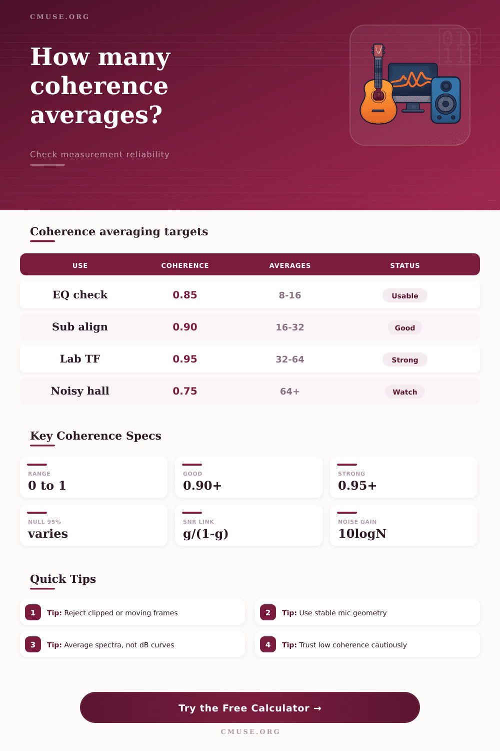
Signal-to-noise ratio and coherence are easily understood as well. Adding uncorrelated energy to the mix decrease coherence. Decent signal dominance would be represented by a coherence value around point nine. Getting into the nineties takes quite a bit more signal compared to noise level. As you see in the reference table on the page, random numbers generates very deceptive coherence results because low averages can produce very high coherence levels. Setting a reasonable confidence limit makes all the difference.
What if your measured coherence number fall below this random number limit? The trace is statistically worthless. There’s no such thing as an EQ’d ghost. These inputs deserve attention because practical measurement scenarios show their need.
Low frequency coherence is one such area where room equalization can struggle. Traffic noise or HVAC rumble will inflate the noise floor without providing significant energy within signal itself. Here, a larger FFT size will serve to reduce the bandwidth of each bin, so it increase the signal-to-noise ratio per bin and improves coherence as a naturaly side effect.
Another challenge is subwoofer alignment, in which case long decay times smears the impulse response, killing coherence in higher frequencies. The trick here is to realize that you’re not battling the software settings; you’re fighting physics of the room. Good measurements are destroyed by source stability. No amount of averaging would of recover from a wobbling mic stand or a vibrating speaker cabinet.
Frame rejection is a feature, not a bug. Let your analyzer throw away bad frames. Thirty clean averages is worth more than sixty contaminated ones. You’ll just end up diluting your signal with non-linear artifacts.
Look at the results and concentrate on the bands you’re going to spend your time listening to. Don’t waste your time chasing perfect numbers out in ultrasonic range where nobody cares. Keep in mind, trust your setup more than your display. In a noisy situation a trace may appear too good to be true; it most likely is.
The guardrails of coherence prevent this from becoming phantom data. After confirming that the coherence holds for the effective averages and within the confidence limits, begin adjusting filters. A pretty curve without coherence is simply colorful noise, ready to spoil system tuning. Control the environment, keep the geometry constant and let the statistics do the work before you rely on any one point on the graph.