FFT Bin Size Calculator
Calculate FFT frequency-bin spacing, nearest-bin error, effective window bandwidth, time span, hop timing, and musical pitch accuracy for audio spectrum analysis.
Choose a real audio-analysis scenario to load a sensible starting point. The calculator separates raw FFT bin size from effective bandwidth, because window shape and zero padding change how a spectrum display behaves.
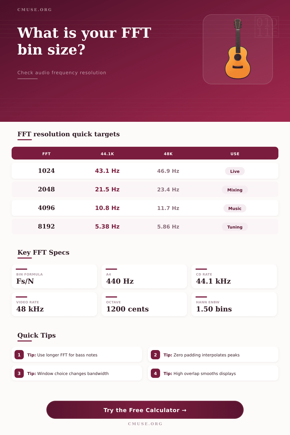
Formulas used: bin size = Fs / FFT size; display bin = Fs / (FFT size x zero padding); effective noise bandwidth = bin size x window ENBW; hop time = window samples x (1 - overlap) / Fs.
Calculation Breakdown
| FFT size | 44.1 kHz bin | 48 kHz bin | 96 kHz bin | Approx. time at 48 kHz | Typical audio use |
|---|---|---|---|---|---|
| 512 | 86.13 Hz | 93.75 Hz | 187.50 Hz | 10.67 ms | Fast live meters and rough transient displays |
| 1,024 | 43.07 Hz | 46.88 Hz | 93.75 Hz | 21.33 ms | Responsive spectrum analyzers and speech views |
| 2,048 | 21.53 Hz | 23.44 Hz | 46.88 Hz | 42.67 ms | General mix analysis above the low bass |
| 4,096 | 10.77 Hz | 11.72 Hz | 23.44 Hz | 85.33 ms | Musical harmonics, resonances, and vocal formants |
| 8,192 | 5.38 Hz | 5.86 Hz | 11.72 Hz | 170.67 ms | Bass fundamentals and tuning checks |
| 16,384 | 2.69 Hz | 2.93 Hz | 5.86 Hz | 341.33 ms | Low-frequency mastering and room mode inspection |
| 32,768 | 1.35 Hz | 1.46 Hz | 2.93 Hz | 682.67 ms | Fine pitch or sub-bass measurement when latency is acceptable |
| Window | ENBW | Main-lobe width | Highest sidelobe | Amplitude behavior | Good use |
|---|---|---|---|---|---|
| Rectangular | 1.00 bins | 2 bins | about -13 dB | Sharpest bin spacing, worst leakage | Coherent test tones exactly on a bin |
| Hann | 1.50 bins | 4 bins | about -31 dB | Balanced leakage and resolution | Music spectrum and spectrogram work |
| Hamming | 1.36 bins | 4 bins | about -43 dB | Better first sidelobe than Hann | Speech and steady instrument tones |
| Blackman | 1.73 bins | 6 bins | about -58 dB | Cleaner side leakage, wider peaks | Separating quiet harmonics near loud ones |
| Blackman-Harris 4-term | 2.00 bins | 8 bins | about -92 dB | Very low sidelobes, broad peak | Low-level artifacts and mastering checks |
| Flat top | 3.77 bins | 10 bins | about -93 dB | Strong amplitude accuracy, widest peaks | Level measurement of isolated tones |
| Source or task | Frequency target | Useful bin goal | Suggested FFT at 48 kHz | Window choice | Reason |
|---|---|---|---|---|---|
| Kick drum fundamental | 45-80 Hz | 5-10 Hz | 8,192 or 16,384 | Hann or Blackman | Needs enough cycles to locate low-end pitch and ring |
| Electric bass low E | 41.20 Hz | 2-5 Hz | 16,384 or 32,768 | Hann | Small Hz changes are musically large in the low register |
| Guitar open A | 110.00 Hz | 2-6 Hz | 8,192 or 16,384 | Hamming or Hann | Stable fundamentals need longer windows than pick noise |
| Piano A4 and harmonics | 440 Hz | 5-12 Hz | 4,096 or 8,192 | Hann | Balances pitch detail with readable harmonic movement |
| Vocal vowel formants | 500-3,000 Hz | 20-50 Hz | 1,024 or 2,048 | Hamming | Formants are broad enough to use shorter windows |
| Cymbal or hiss texture | 6-16 kHz | 50-200 Hz | 512 or 1,024 | Hann | High-frequency work usually values speed over fine bins |
| Mains hum diagnosis | 50 or 60 Hz | 1-3 Hz | 16,384 or 32,768 | Blackman-Harris | Low sidelobes help reveal harmonics and nearby noise |
| Note or range | Frequency | 1 cent at that pitch | 5 cent span | FFT bin needed for 5 cents | Real-world caution |
|---|---|---|---|---|---|
| Bass E1 | 41.20 Hz | 0.0238 Hz | 0.119 Hz | Over 403k at 48 kHz | Peak interpolation or pitch tracking is better than raw bins |
| Guitar E2 | 82.41 Hz | 0.0476 Hz | 0.238 Hz | Over 201k at 48 kHz | Long FFTs improve view but do not replace a tuner algorithm |
| Middle C C4 | 261.63 Hz | 0.151 Hz | 0.756 Hz | Over 63k at 48 kHz | Useful for slow analysis, not responsive live display |
| A4 concert pitch | 440.00 Hz | 0.254 Hz | 1.27 Hz | Over 38k at 48 kHz | Zero padding helps read a peak but not separate two tones |
| Soprano C6 | 1046.50 Hz | 0.604 Hz | 3.02 Hz | Over 16k at 48 kHz | Higher notes need fewer samples for the same cent accuracy |
| Project | Sample rate | FFT / window | Bin size | Time span | Starting note |
|---|---|---|---|---|---|
| Podcast voice cleanup | 48 kHz | 2,048 / Hamming | 23.44 Hz | 42.67 ms | Good for formants, hum needs longer FFT |
| Home mix spectrum | 44.1 kHz | 4,096 / Hann | 10.77 Hz | 92.88 ms | Readable balance without feeling too sluggish |
| Live room analyzer | 48 kHz | 1,024 / Hann | 46.88 Hz | 21.33 ms | Fast motion, broad frequency bins |
| Mastering low-end check | 96 kHz | 32,768 / Blackman-Harris | 2.93 Hz | 341.33 ms | Stable low-end display with slow response |
| Instrument tuner view | 48 kHz | 16,384 / Hann | 2.93 Hz | 341.33 ms | Visual estimate only; use interpolation for fine tuning |
| Drum transient spectrogram | 48 kHz | 512 / Hann | 93.75 Hz | 10.67 ms | Preserves timing at the expense of bass detail |
When you look at a spectrum analyzer, you’ll see peaks of data, but perhaps not know they’re limited by the number of samples provided to the math. Even experienced engineer get tripped up by the power of the Fast Fourier Transform and its forced trade-off between time and frequency. If your window on the FFT is too short, then you don’t have sufficient cycles of your waveform to resolve closely spaced tones so your frequency resolution suffers. Conversely, if you make the window too long, then you lose temporal precision and actualy miss transients all together.
Calculating precisely what resolution your bin size will give you with your chosen sample rate and target pitch is key to finding right balance. There is the raw bin spacing, which is simply dividing the sample rate by the FFT length. Underneath that, there is some complexity. If you have a 2048-point FFT at a 48 kHz sample rate, you’ll find about 23 Hz between each bin center. That sounds precise enough, right? Well how about trying to tune a low E bass note at 41 Hz? Half a bin means a big ol’ pitch shift. The problem lies in understanding whether or not the settings you’ve selected is capable of handling the cents of error you’re concerned with.
Understanding the FFT Trade-off
Most folks think that zero padding the FFT will fix things, because it adds extra points to the graph so it looks smoother. But it doesn’t create any new information; it only fills in the gaps between existing data. So while the graph looks smoother, it won’t be able to separate two distinct frequency that fall on either side of its resolution limit.
And then there’s a further compromise via window functions. After all, if you have a perfect amplitude measurement, you won’t have good frequency resolution either. If you use a rectangular window, you’ll get very narrow frequency bins but terrible spectral leakage, as energy spills over into adjacent frequencies so much that your display becomes a mess of side lobes: If instead you choose a Hann or Blackman-Harris window, you can reduce the spectral leakage a lot. It will still be present, but not as extreme than before because these windows taper the edges of the signal slice you are looking at. But you also widen the main peak doing so. That means that the actual effective bandwidth you’ve got is wider than just the size of each bin indicates.
That is why the tool displays the equivalent noise bandwidth. This is frequently a better number to look at if you are trying to identify quieter artifacts around louder fundamental tones, for instance.
In real world audio work, pitch and timing go hand-in-hand. You double the FFT size to get greater frequency detail (smaller bin width). This doubles the amount of time being analyzed which decreases the accuracy of the timing information. At 48 kHz, a 32768- point window represent almost seven-hundred milliseconds of audio. For a snare snap or kick drum hit, that’s an eternity. Because the energy is averaged across too many frames, the attack becomes smeared into a muddy blob. You may end up with the perfect frequency data on something that has already happen.
The solution to this lies partially in the overlap setting. Instead of jumping the window forward its entire length, overlap shifts the window slightly. This provides more frequent updates without losing the detail you gain from a longer analysis duration. In practical mixing terms, this means picking a setting that hits the sweet spot between these competing requirements. When analyzing a mix bus for the most part, a 4096-point FFT is typically fine for revealing instrument harmonics and vocal formants. It also won’t freeze the display in time.
Where you’re digging into really low frequencies (sub bass) or resolving very slow waves like measuring room modes, something like 16384 points or larger is probably required to sort them out properly. But again, the reference tables on the page set this all out in clear detail for commonly used sample rates so you don’t have to guess.
You are basically making a decision about whether you want to know when a frequency began playing or where it sits in the spectrum. Understand that compromise, and your settings will no longer feel like a guess but more like an engineer’s choice. Stop trying to measure everything down to the nth degree all at once and the mountain of data begins to get manageable, you should of known that.